Farm Operations Management
Vertical Farm Crop Schedule: Revise Often to Ship, Seldom to Grow
Articles for Farm Operations Managers
“Build the schedule around full production capacity, and just fit shipment and staffing to it”—is that not how you think about your crop schedule? Build it that way, and every week the numbers stop adding up somewhere. You have a surplus on the shipment side, complaints come in from the staffing side, and you spend your time cleaning up after it. You assume the schedule on paper isn’t precise enough, so you rebuild it in finer detail. But no matter how fine you make it, the drift doesn’t go away. If that’s the case, perhaps the place you’re suspecting is simply the wrong one.
I have spent a long time growing and launching leafy greens such as lettuce in PFAL vertical farms, and a good share of the situations where a plan stops working came not from the fineness of the schedule on paper, but from the moment things that move at different speeds were tied into a single line.
Plan drift is a problem of three clocks, not precision
There are any number of situations where things don’t run as the schedule on paper says they should. Watch closely and you notice that the drift doesn’t come in just one kind. The swings of surplus and shortage in shipment move in fine, week-by-week steps, whereas cultivation itself is much slower: even when you change the rhythm of final planting, the result doesn’t show up until weeks later. And the ebb and flow of labor peaks at yet another timing. Within the same “plan,” things of different speeds are mixed together—have you not felt that?
This is not just one particular person’s impression. As far as I can see, most cases where a plan stops working start here. We call it “crop schedule” in a single word, but inside it there are at least three different clocks. Shipment is pulled by demand and sways in fine week-by-week steps. Cultivation is the cycle of a living thing, so even when you act, the reply doesn’t come back until weeks later. For leafy lettuce, a single plant takes about 35 days from seeding to harvest. Even when you intervene, the effect doesn’t reach the shelf until a cycle later. The ebb and flow of labor moves on peaks different from either of those.
The problem is putting these things of different speeds onto the same scale of a single schedule on paper. Match the fast swings and the cultivation side gets jerked around; match the slow cycle and shipment lets orders slip. So the drift is not a problem of the schedule’s precision. It is a structural problem of forcing three things that should each turn separately to synchronize.
“Try to grasp it as a single line and it drifts”—this comes up in the same form on the research side too. When you try to predict the weight of vertical farm lettuce at harvest from the apparent size at one single moment, the correlation tops out at 0.45. But add a feature that spans time, such as leaf movement, and it rises to 0.74 (see 1). That leaf movement itself has a periodicity linked to the light-dark cycle (see 1). Look not at one still frame but at the flow of time—that is, at the cycle—and reality reads better. The plan is the same: act on the shipment count of one given week alone and you miss. Only when you view it as a wave, as a cycle, does reality begin to read.
How to place buffers so the three axes turn separately
Told there are three clocks, you may find it falls into place. But here one snag remains. Even told they should turn separately, in practice the three pull on each other. Try to answer the swings in shipment and you’ll want to fiddle with the rhythm of final planting; when a harvest peak comes, labor gets dragged along to it too. What, concretely, does keeping the right distance mean when you turn them separately? If you don’t bundle them into one line, what do you watch to mesh the three together?

Turning shipment, cultivation, and labor separately means deliberately placing a “buffer” between the three. Connect them directly, and a fast swing shakes the slow cycle as it is. That is exactly why you insert a buffer in between, so that one side’s shaking doesn’t pass straight through to the other. Concretely, what you can place on the shipment side is how long plants can wait on the shelf for the right harvest point, how far up or down you can flex the grades you ship, and the room to adjust contract quantities. What you can place on the cultivation side is the latitude in the spacing of final planting; on the labor side, spare capacity. Let me add one caveat from the field here: fresh leafy greens keep poorly, so the latitude to hold them in stock for days on end is limited. So the buffer on the shipment side is held less by “stocking inventory thick” than by how far you can swing the right harvest period on the shelf back and forth, and which grades you can divert to shipment. Note, too, that these are not the only ways to take a buffer. To be precise, each axis has finer ways to hold one, but to keep the discussion clear, here I’m limiting it to the representative one for each axis.
The clue for meshing them together is not the schedule on paper itself. It is how much of that buffer is left right now, or how much it’s drawn down. Absorb the swings in shipment with the window of the right harvest period and the latitude of grades, and when that room is about to run out, adjust the final planting rhythm on the cultivation side. Absorb harvest peaks with people’s spare capacity. Rather than synchronizing the three on the same scale, watch how much buffer is left between each of them and adjust only the one that’s nearing its limit.
What to be careful of here is that the cultivation-side remedy doesn’t make it in time if you wait “until the buffer runs out.” Increase final planting after the buffer absorbing shipment has dried up, and that plant doesn’t reach the shelf for about 35 days. That’s a move made too late to help. So the cultivation axis alone you move ahead, by the amount of lead time to harvest, without waiting for the buffer to run out. Watch the slope of the buffer’s decline and act before it bottoms out. Where the shipment-side watch looks at “how many right now,” the cultivation side looks at “going on like this, will there be enough at the far end of the lead time”—that is the difference.
Rather than fixing everything all the way to the end with a single line, let the three clocks each turn at their own speed and monitor only the buffers at the boundaries. That is the kind of distance you keep.
That labor is an axis separate from production can be backed from the management-data side too. An industry survey of greenhouses under protected cultivation (tomato) observed a peak in profitability around 6,000–8,000 m2, and reported that the main challenge in running it sustainably is “stable production and the procurement and allocation of labor” (2017, see 2). This is a survey of fruit vegetables and greenhouses, a different type from the PFAL and leafy greens I’ve seen in the field, but the point that labor is not merely a variable subordinate to the production process carries across types. Profitability is largely driven not by using production capacity to the fullest, but by how you reconcile production and labor. I consider labor an axis to set apart and fit to, on its own.
Choosing the axis to set as the baseline
Try to shift cultivation to fit the shipment plan or people’s convenience, and the rhythm of growth just won’t bend that easily. Have you not had this experience? Of the three clocks, the cultivation cycle alone is roughly fixed by light and temperature, and can’t be moved as freely as shipment or labor. So in practice an order naturally emerges: “set the axis that’s hard to move as the baseline, and fit the movable axes to it.” Conversely, a facility that wants to put orders first may set shipment as the baseline. What you set as the baseline cycle changes how you build the plan itself.
Of the three, the cultivation cycle is the hardest axis to move. Light, temperature, and the rhythm up to harvest can’t be bent by the convenience of people or orders. So set cultivation as the “baseline clock” and fit shipment and labor on top of it. This is the way with the least strain.
What matters here is that no matter what you set as the baseline, the baseline doesn’t directly move the others. Even with cultivation as the foundation, you absorb the swings in shipment with the window of the right harvest period, and absorb labor peaks with spare capacity. The way of placing buffers we saw in the previous section doesn’t change here either.
It’s the same when an order-first facility sets shipment as the baseline. This time you give the cultivation side a thick buffer—the latitude of final planting—and let it soak up the swings. A facility that wants to level out employment sets the amount of work people can move as the baseline, and draws shipment and cultivation toward it. Order-led, production-led, or labor-led—whichever you choose as the baseline, the logic doesn’t change. To change the baseline is to choose anew which clock to fix and which buffer to thicken. Set the hardest-to-move axis as the baseline and shift the cushion onto the movable axis. The order always comes out this way.
That said, in facilities with heavy contract sales, this asymmetry can flip. When shipment quantity is more or less fixed by contract, shipment becomes the most stable axis instead, and what sways is the production side—yield and the variability of growth. In that case you hold a thick buffer on the production side and fit cultivation to the stable axis of the contract. What is most stable and what sways most in your own facility changes with your contract makeup.
And even though you set the cultivation cycle as the baseline clock, that baseline isn’t completely rigid either. Lettuce growth rises and falls with light intensity, but the optimum point shifts with the combination of photoperiod and nutrient solution concentration, and there is no single value that is “the one optimum” (see 3, 4). Even within the axis you set as the baseline, there is latitude left to choose. Hard to move is not the same as impossible to move at all.
Making slack in the hard-to-move cultivation axis
Told that facilities setting shipment as the baseline thicken the cushion on the cultivation side, does that not catch a little? The cultivation cycle is fixed by light and temperature, and should be the hardest of the three axes to move. And yet you can give that hard-to-move axis a buffer—the latitude of final planting. It’s a slightly strange story. What, concretely, does it mean to make a buffer in something hard to move? Is the supposedly stiffest axis in fact the place where you can add the most cushion?
To put the conclusion first: that’s exactly it. The harder an axis is to move, the more cushion you can add. The cultivation cycle itself—that is, how many weeks a single plant takes from seeding to harvest—truly can’t be moved. But “when to sow” and “in how many batches to sow” can be moved. Spreading these out is the latitude of final planting.
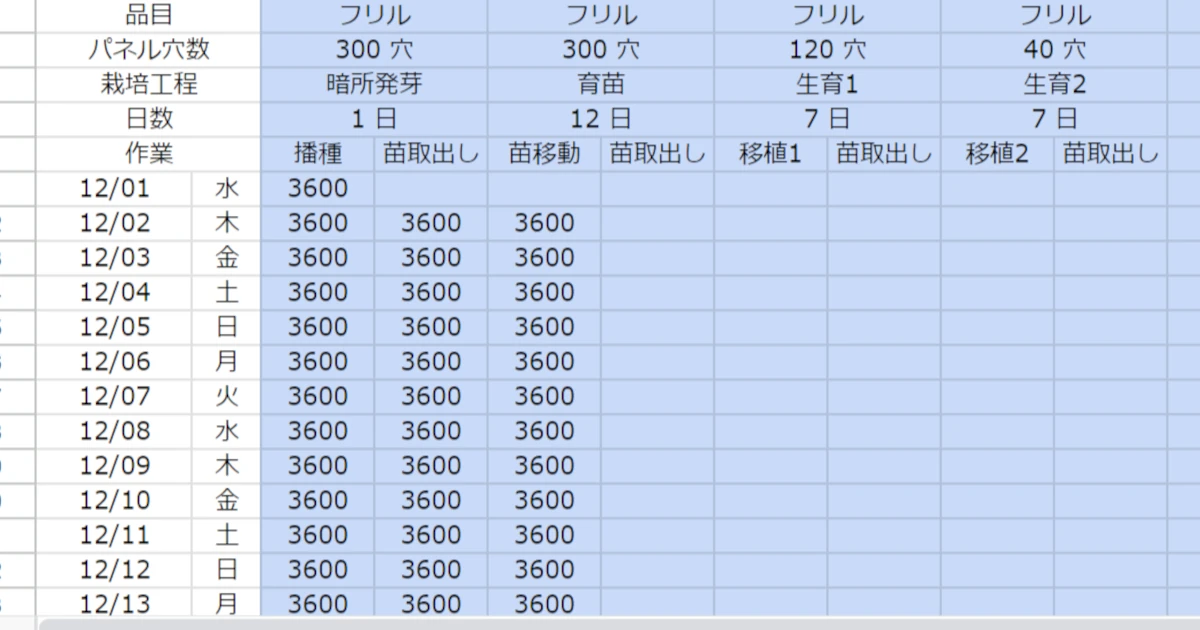
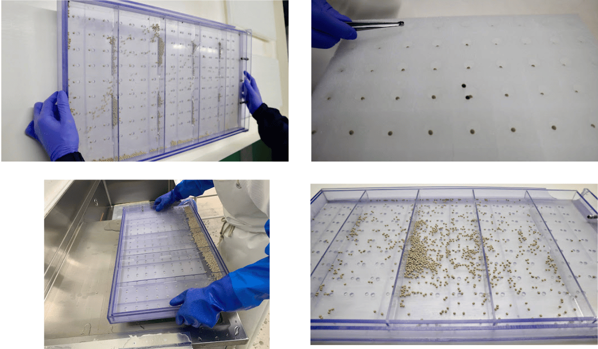
Sow a large amount all at once and harvest concentrates at a single point too, with no way to fit it to the swings in shipment. But sow a little at a time on a staggered schedule, and on the shelf “plants about to enter their harvest period” and “plants nearly ready to harvest” line up in steps. Weeks when shipment rises, you harvest earlier; weeks where there’ll be a surplus, you hold off a little. That kind of latitude is born. This drops straight into seeding design in the field. If, say, a contract is 5,000 plants a day, rather than sowing them all in one day, you split the sowing across several days so that roughly the same amount is ready to harvest every day. A factory that grows in multiple stages divides shelves into propagation, early, mid, and late, and always keeps several days’ worth of plants in stock at each stage. Set it up this way and you can adjust: a week when shipment swells, you bring plants forward from the late shelves; a week you want to rein in, you let them sit a little. With a single day’s batch sowing, that latitude simply doesn’t exist.
What’s hard is the cycle of each individual plant; what’s soft is how you scatter those plants along the time axis. By staggering and overlapping units you can’t move, you get a buffer as a whole. The reason the hardest axis becomes the place where you can add the most cushion is that hardness and arrangement are separate matters.
Something close to this read—what’s hard is the cycle of each individual plant, what’s soft is the arrangement along the time axis—can be seen in research on how light is distributed too. This is an example from a different area, not about the allocation of seeding itself, but the structure “change the way it’s distributed without changing the total, and the result moves” is shared. For instance, with ‘Little Gem’ lettuce grown in a greenhouse with supplemental lighting, distributing the same total amount of light weakly over a longer time, rather than strongly in a short time, increased biomass and raised the conversion efficiency per unit of light too (see 5). That said, this is under greenhouse-plus-supplemental-light conditions, and the same study also reports a quality trade-off: stretch the photoperiod too far and tipburn increases. It isn’t a simple matter of “the longer the better.” Even in the closed environment of a PFAL, there’s a result that moving the light intensity over the day to match fluctuations in electricity prices cut lighting cost by about 12% without dropping yield, as long as the total was kept (see 6); and the same study further found that distributing light by ramping it up in stages, rather than holding it constant, raised dry weight by about 12% for the same total (see 6). There is also research that examined the very method of shifting electricity use to match demand and price (see 7). The types and subjects differ, but it does reinforce that there are situations where distribution matters more than the total.
Vary the rhythm of reviewing buffers with the speed of the wave
The idea of adjusting by watching how much buffer is left probably sits well. But here one question arises. When, and how often, should you look at how much is left? Shipment moves in fine week-by-week steps. Cultivation’s reply is weeks away. Labor has yet another peak of its own. Peering at all three at the same interval feels off, yet if you vary the frequency, now it seems you might miss something. Does the rhythm of looking come to differ for each buffer?
How often to look is determined by the speed of the wave that buffer is absorbing. The faster the wave a buffer is absorbing, the shorter the interval—and what you look at is only how much is left. For the window of the right harvest period that absorbs shipment, you peer every day or every few days at “how many plants on the shelf can swing back and forth right now, and is that dwindling.” At this point you don’t make the judgment to move the baseline. You just confirm where the leftover is right now.
A buffer absorbing a slow cycle is fine on a long interval. But what you look at differs. The cultivation side, which holds the latitude of final planting, shows no response even if you measure it weekly, so once every few weeks you review the baseline itself: “is the current spacing of final planting even right?” Not confirming how much is left, but inspecting the setting. And this inspection you run before the buffer dries up—earlier by the amount of lead time. The cultivation side alone allows no catching up after the fact.
In other words, even the same “looking” has two layers. The fast buffer, short and frequent, for how much is left; the slow buffer, on a long interval, for the setting. Even out the intervals and the fast one gets missed while the slow one gets needlessly jostled. The rhythm of looking at each buffer may be varied to match the wave it’s taking.
The way a buffer draws down points straight at “which axis’s setting was too lax.” If the window of the right harvest period is always tapering, the cultivation side’s final planting spacing isn’t keeping up with the swings in shipment. If people’s spare capacity is always strained, the labor-side estimate isn’t absorbing the harvest peaks. If shipment keeps letting orders slip, the buffer placed on the shipment side is itself thin. Rather than lumping drift together as “a lax plan,” you can isolate the axis of the cause by which buffer starts to crumble first. This, I feel, is the greatest practical benefit of seeing things in three axes.
That said, chasing how much buffer is left like this, spacing seeding by counting back from the delivery date, allocating the number of plants to each stage—building all of this from scratch every time is fair work. I’ve made the crop schedule template I used in the field public on this site, so it should serve as a foothold for grasping how the formulas are put together. But it’s not something you can use as is. The number of plants, the turnover, and the yield differ by factory, so to actually run it you have to remake it to fit your own environment. First, for study’s sake, download it from here and have a look inside.
Drift the three axes can’t absorb, and the stance to hold from the start
By now we’ve laid out the three clocks and how to view the buffers between them. Lastly, let me draw one line. Everything up to here was a framework of “absorbing the drift within the range the three axes turn, through how you place buffers and the rhythm of review.” But there is also a kind of drift that no amount of thickening the buffers can absorb. For instance, when demand itself is structurally and continuously thinning, or when the level of fixed costs sits somewhere that cycle adjustment can’t reach. Such drift is not a matter of how you build the plan; it’s a matter of re-examining sales channels and contract terms, or the very scale of the equipment, and it’s a different arena. It’s a problem outside the frame of “meshing the three axes together.”
This boundary line—the kind of drift buffers can’t absorb—becomes clear when you look at the sensitivity of profitability. The profitability of a lettuce vertical farm is brutally sensitive to selling price. By one estimate, a mere fixed-percentage drop in selling price from current levels sends the scale needed to break even shooting up sharply, and as the drop grows, it balloons to a scale that isn’t realistic (premised on advanced cultivation technology and the current cost structure; see 8). That very sensitivity—a small downward swing in price moving the required scale by a lot—bears on the side building the plan. This is no longer a width you can absorb with the spacing of final planting or the right harvest period on the shelf. It’s the case where a different cycle—price and demand—drifts structurally.
On the cost side too, there are external cycles outside the buffer. In a PFAL vertical farm, what mainly bears down is electricity. An industry survey shows electricity’s share of PFAL costs rose from 19% in fiscal 2021 to 24%, and the breakdown of that electricity cost is lighting 58%, HVAC 31%. The year-on-year electricity cost structure even spiked to 131% in fiscal 2022 (fiscal 2025 survey, see 9). If the unit price of electricity moves greatly from the outside, the spacing of final planting can’t absorb it. The same cycle of an “external price shock” occurs in greenhouses not on electricity but on the fuel-oil side. There is a point that high crude oil prices and a weak yen could push fuel costs in protected cultivation to record levels (see 10); the source differs, but the cycle of prices being pushed up from outside is common across types. PFAL readers, I think, do well first to view the external fluctuation of their main cost—electricity—as a matter outside this buffer. Once it gets to this, you enter the territory of re-examining not how you build the plan, but sales channels, scale, and procurement itself.
For someone newly launching, what changes by holding this three-axis way of thinking from the start? What changes most is “what you suspect when things drift.” Without the three axes, every time things drift you try to raise the precision of the schedule on paper, making the single line finer and finer. But that is the direction of forcing things of different speeds into one, and it usually hits a wall. Know from the start that there are three clocks, and at the launch stage you can build “where to place the buffers” into the design. The window of the right harvest period on the shelf, the spacing of final planting, people’s spare capacity—these are hard to add later, but at the start you can work them in without strain. Whether you can see a plan not as a line drawn all the way to the end but as a mechanism that keeps turning while it takes the shocks: that is the entry point that shifts. Hold that stance and you should be able to look at even the first drift calmly—not as a failure, but as a signal that the three axes have begun to move.